Infinity is a fascinating idea and it is behind some of the most beautiful results in mathematics. Much of this beauty is accessible to everyone, brought to us by the brilliant Georg Cantor using simple arguments that require little math. I hope to show some of this goodness to people who haven't seen it before. Here we go.

Imagine a shepherd tending a flock of a few dozen sheep. In the morning, the sheep get out of the farm to do sheepish things. In the evening, the shepherd wants to make sure he got all his sheep back. One problem: he can't count. What's a shepherd to do? One solution would be to keep track of the sheep as they go out. For example, he could throw a pebble into a bucket for each sheep leaving the farm. In the evening, a pebble goes out for each returned sheep. At any given time, the number of pebbles in the bucket is exactly equal to that of outstanding sheep. You can picture the sets of sheep and pebbles like so:

Each sheep is paired with a distinct pebble and there are no left overs on either side. In set theory this is a bijection. Even though the sheep have not been counted, we know the sets have the same number of elements. They are equivalent in a way, not because you eat pebbles or throw sheep, though I suppose you could, but because of the bijection. If you accept this premise, which is reasonable enough, then you're in for some fun. Interesting things happen when we use bijections to compare sets nobody can count: the infinite sets. For example, let's compare the natural numbers (1, 2, 3...) to the even natural numbers (2, 4, 6...). It sounds like we should have less even numbers, but lo and behold, we get this:

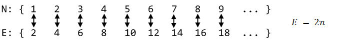
Every natural number has been paired with a distinct even number. No left overs. Strangely, these sets are equivalent. It turns out many sets are equivalent to the natural numbers; we call these sets denumerable. For example, the set of Turing Machines is denumerable because there are infinitely many machines and they can each be fully described by a distinct natural number. The integers are yet another example:

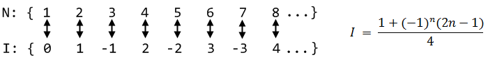
Some people see these results as trivial: their intuitive notion is that any "infinity" must be the same. Others see a paradox. How can a part of something be equivalent to the whole? Let's try to give everyone a paradox by finding a set that is not denumerable. How about the rationals? Surely there must be more fractions than natural numbers! Right? Cantor probably thought so, until he discovered a procedure to enumerate the rationals:

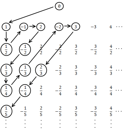
Starting at the top and following the pattern, this procedure hits each rational number once. As it moves along, we can associate successive natural numbers with each hit. Here are the first few pairings:

It is pretty clear that the arrangement above covers all of the rationals, but the crucial point is that Cantor's pattern will reach any given rational in a finite number of steps. The zigzag is important: if we go off in a single direction (say, across the first row to the right) then we get stuck in the infinitude of that row alone, and there would be rationals left over. The zigzag delivers us from that evil. This argument does not produce an equation for a bijection, but since it builds a listing that contains every rational number, it shows they are denumerable. Conversely, if a set is denumerable its elements can be put into a listing where each element is paired with a natural number.

(As an aside, the 1999 paper Recounting the rationals establishes a precise bijection by using a tree to generate all fractions in reduced form. The tree has all sorts of magical properties, cool stuff. It's an accessible paper, plus Brent Yorgey wrote a great walk through of it.)

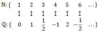
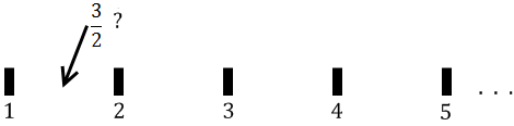
All of our sets so far have been denumerable, except for the sheep who were finite. At this point, Cantor might have wondered if maybe there is only one infinity. But then again, if you build a number line using the sets we have seen so far, you end up with holes. The naturals are mere dots on the number line, most fractions fall in a hole:

The rationals, on the other hand, are dense. Between any two given rationals, there is another rational (an infinite number of them actually). Yet the rational number line also has holes, which are the irrational numbers. Below is a famous irrational number, on whose account its discoverer was allegedly drowned at sea, shown along the rational number line:

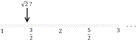
Irrational numbers cannot be expressed as a fraction; moreover, when written out as numbers using positional notation (say, as decimal numbers) their digits never settle into any kind of periodic pattern. Fractions, by contrast, eventually settle into a pattern when written out (e.g., 0.333..., 0.25000...). All of the rationals plus all of the irrational numbers make up the real numbers. And those guys form a number line free of holes. Any point in the number line is a real number, any crazy sequence of digits you come up with is a real number. It's the continuum. You might get the impression that irrational numbers are rare, oddballs among the familiar rationals, but that's not the case at all. The sparse number line above is an attempt at visualizing that fact, in addition to showcasing my superior preschool MS Paint skillz. The reals are a vast ocean of irrationals pointed here and there by a fraction, and we'll see why.

So now Cantor pits the real numbers against the naturals. He shows that even a section of the reals - the interval between 0 and 1 - is not denumerable. He uses a proof by contradiction, which is a common way to show that something cannot be true. It goes like this: suppose there is a way to enumerate the reals between 0 and 1. Then there is a listing containing every real number in that interval, each one associated with a different natural number. It might look like this:

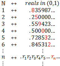
The actual numbers shown above are not important, since the complete list is infinite and has every real number in the interval. Some of the reals up there are clearly rationals and have settled into a periodic pattern (0.250... and 0.500...). The others look pretty random, they could be irrational or maybe they haven't settled into their periodic patterns yet. Either way, for each number the digits go on indefinitely, rationals in a pattern (possibly of zeros) and irrationals randomly.

Notice how the numbers in red form a diagonal, which is itself infinite. Let's build a number using that diagonal. Going down the list, for each row we pick a digit that is different than the digit in red. For example, we could add 1 to each digit (9 becomes 0, no carry). You can use any rule as long as the digit is different. Here are the first few digits we get by adding 1 to the red diagonal digits:

The digits of this number p are random and go on infinitely; it is a real number. But due to how we have defined p, it is different from every other number in the list. It differs in at least one digit. Even though the list is infinite, this number is not in it! But then, this list was supposed to have all real numbers so we have a contradiction. Hence our initial assumption must be false; the reals are not denumerable.

The notion of different infinities was a revolutionary one in mathematics. It is a stunning result which ignited the mother of all mathematician flame wars. This was actually the second proof Cantor offered for the non-denumerability of the continuum. The first proof is also valid, but slightly more technical. Cantor's diagonal argument however is amazingly simple and highly original, as brilliant as its conclusion. It went on to feature prominently in other intellectual landmarks. Alan Turing used it while proving that a Turing Machine cannot predict the behavior of other machines (specifically, predict whether another machine is "cycle-free", which is now known as the Halting Problem). Gödel used it in his Incompleteness Theorem discussed in Gödel, Escher, Bach. Diagonalization is crucial in recursion theory and complexity theory.

In order to capture these new concepts, Cantor proposed cardinality as a measure of how numerous a set is. A finite set's cardinality is simply how many elements it has, say 49 for our set of sheep. But the cardinality of an infinite set is expressed by a transfinite number. To make them more esoteric, Cantor used the Hebrew letter aleph for these numbers. By definition, the naturals took aleph zero, , for their cardinality. Every denumerable set has cardinality . The cardinality of the reals was defined as c, and Cantor spent years trying to discover whether c = , that is, whether the cardinality of the reals is the 'next bigger one' after the naturals. So that explains the name in Mona Lisa Overdrive and also the handle for Aleph One, who wrote the classic paper on stack buffer overflows during the Phrack renaissance.

This concludes our first foray into the infinities. There's way too much to talk about. If there's interest I'll write a follow up to see where else infinity leads us. Iterative rather than upfront blogging :) Meanwhile, Journey Through Genius is a great book that does for many theorems, including Cantor's, what I did on this post. Only much better. Thanks for reading!

[31 Comments](/comments/counting-infinity.html)

For 2,000 years scholars held that heavier objects fall faster than lighter ones, partly because Aristotle couldn't be bothered to take 2 minutes to experiment. Hell, he even wrote that men have more teeth than women. Isn't that crazy? And yet, people often rely on this kind of fact-free reasoning to arrive at conclusions about computer performance, among other things. Worse, they spend their IT budgets or sacrifice code clarity based on these flawed ideas. In reality computers are far too complex for anyone to handle performance problems by "reasoning" alone.

Think about a routine in a modern jitted language. Right off the bat you face hidden magic like type coercion, boxing, and unboxing. Even if you know the language intimately, unknowns are introduced as your code is optimized first by the compiler, then again by the JIT compiler. It is then fed to the CPU, where optimizations such as branch prediction, memory prefetching and caching have drastic performance implications. What's worse, much of the above can and does change between different versions of compilers, runtimes, and processors. Your ability to predict what is going to happen is limited indeed.

To take another example, consider a user thinking of RAID-0 to boost performance. Whether there are any gains depends on a host of variables. What are the patterns of the I/O workload? Is it dominated by seeks and random operations, or is there a lot of streaming going on? Reads or writes? How does the kernel I/O scheduler play into it? How smart are the RAID controller and drivers? How will a journaling file system impact performance given the need for write barriers? What stripe sizes and file system block sizes will be used? There are way too many interdependent factors and interactions for speculative analysis. Even kernel developers are stumped by surprising and counterintuitive performance results.

Measurement is the only way to go. Without it, you're in the speculation realm of performance tuning, the kingdom of fools and the deluded. But even measurement has its problems. Maybe you're investigating a given algorithm by running it thousands of times in a row and timing the results. Is that really a valid test? By doing so you are measuring a special case where the caches are always hot. Do the conclusions hold in practice? Most importantly, do you know what percentage of time is spent in that algorithm in the normal use of the application? Is it even worth optimizing?

Or say you've got a fancy new RAID-0 set up. You run some benchmark that writes large globs of data to the disk and see that your sustained write throughput is twice that of a single disk. Sounds great, too bad it has no bearing on most real-world workloads. The problem with the naive timing test and the benchmark is that they are synthetic measurements. They are scarcely better than speculation.

To tackle performance you must make accurate measurements of real-world workloads and obtain quantitative data. Thus we as developers must be proficient using performance measurement tools. For code this usually means profiling so you know exactly where time is being spent as your app runs. When dealing with complex applications, you may need to build instrumentation to collect enough data. Tools like Cachegrind can help paint a fuller picture of reality.

For website load times and networks you might use tools like WireShark and Fiddler, as Google did for GMail. In databases, use SQL profiling to figure out how much CPU, reading, and writing each query is consuming; these are more telling than the time a query takes to run since the query might be blocked or starved for resources, in which case elapsed time doesn't mean much. Locks and who is blocking who are also crucial in a database. When looking at a whole system, use your OS tools to record things such as CPU usage, disk queue length, I/Os per second, I/O completion times, swapping activity, and memory usage.

In sum, do what it takes to obtain good data and rely on it. I'm big on empiricism overall, but in performance it is everything. Don't trust hearsay, don't assume that what held in version 1 is still true for version 2, question common wisdom and blog posts like this one. We all make comical mistakes, even Aristotle did. Naturally, it takes theory and analysis to decide what to measure, how to interpret it, and how to make progress. You need real-world measurement plus reasoning. Like science.

10 Comments

Update August, 2013: Stick Shift is a product that implements this on Windows.

This post teaches you how to set up your computer so that you can generate any keystroke or key combination without taking your hands off home row (the ‘asdf’ row of keys). You can then use the arrow keys, page up/down, shortcuts, and more while in regular typing position. It works across applications, allowing you to type and move about much faster. I call it ‘home row computing’ and it’s something I started doing after I learned touch typing.

I’ll explain the idea and give step-by-step instructions for Windows systems. The first step is to do what power users have done all along: reclaim the Caps Lock key. It is a fine piece of keyboard real estate gone completely to waste, like a landfill in the middle of Manhattan. We must also do some key remapping:

The idea is to change Caps Lock so that it can be combined with other accessible keys to produce all of the faraway keys shown above, plus frequent key combinations and anything else you might want. When I say “map to home row” I mean mapping to keys that can be reached while your hands remain on home row. Nearby letter keys are fine too. For example, Caps Lock+j could become the Up arrow and Caps Lock+e could become Alt+F4.

It is common to turn Caps Lock into Control, but we don’t actually want that because nearly all Control+X combinations are already taken by various programs, so we wouldn’t be able to do much remapping. Some Control+X combinations are very high yield (e.g., the copy/paste/cut combos) so we’ll remap those onto home row. I think the best substitute for Caps Lock is the “Apps Key”. Since no software uses it as a shortcut ingredient, we can hijack it without fear. Also, its normal role is to open a right-click context menu, so that’s a useful thing to have on home row as it helps you stay clear of the mouse.

So download SharpKeys, run it, and turn Caps Lock into the Application Key as shown below:

OK, then click “Write to registry”, log off and back on, and you’re in business. The second step is to download the outstanding AutoHotKey to run our remapping script. AutoHotKey is a must have for Windows power users, featured repeatedly on lifehacker. Since it is a full-on automation and scripting engine there are many ways to do things. However its native key remapping syntax (OldKey::RemappedKey) doesn’t work for us here since we want to map key combinations into single keys. But you don’t have to worry about that, you can just download my ready-made script for either the qwerty (normal) keyboard layout or the Dvorak (freak) layout. Put it anywhere in your file system, then create a shortcut to the script in the Programs > Startup folder so it runs when you log on to Windows. By inspecting the script you’ll be able to tweak it for your tastes. Here’s what it does out of the box:

Thanks to AutoHotKey’s eliteness the layout works well in practice. The timing is not quirky at all and there are zero misfires. If you hold down Caps Lock, you can press the other keys repeatedly and they’ll be remapped. Let go of Caps Lock and they’re back to normal. The script also handles modifiers such as Alt and Shift being pressed along with the key combinations. It’s pretty transparent. If you want to actually toggle caps lock, then Windows Key + Caps Lock will do the trick.

It is a joy to have navigation keys on the home row. It makes browsing, programming and writing much smoother. You can fly through dialogs. Having Esc nearby is not bad either. All in all, I can’t imagine going back to a regular keyboard. Given AutoHotKey’s power you can write scripts to handle key combinations so there are many possibilities. I adapted to this thing pretty fast; the symmetries between page up/up arrow, home/left and so on helped a bit. Again, it’s trivial to pick your own bindings, take a look at other ideas for cursor movement and cook up your own scheme if you wish.

Some quick thoughts regarding text editors. When I first did this I was an Emacs user so having a convenient Control key was crucial, but I still think it’s better to turn Caps Lock into the Apps Key instead. Then you can pick and choose your macro bindings between Control and Caps Lock, and given AutoHotKey’s power you have a lot of leeway. I have since switched to Vim (apostasy!!) and never looked back. Vim users will recognize the beauty of having arrow keys on the home row, but will probably barf at the exact key choices I used since jklh is burned into their brains. Just edit the script. You’ll like navigating without switching modes, and Esc on the home row is great for when you do switch. In Visual Studio this works seamlessly without interfering with any of the native shortcuts.

I’ve tried this out on Windows XP, Server 2003, Vista, and Server 2008, both 32- and 64-bit flavors. No problems that I know of, but use it at your own risk. The script works over Putty so the keys are available on the command line and Vim for all of the Unix boxes I use. If you know of similar approaches in other OSes I’d love to hear it in the comments. Hope this is useful!

Update: Amjith pointed me to XKeymacs, a tool that implements the same idea but for emacs keybindings (you could do a similar thing via AutoHotKey, but this is convenient for sure). Also, you guys in the comments are all in favor of Vim-style HJKL bindings, so if anyone makes a script to do that, I’d be happy to host it.

Update 2: Simon Scarfe has posted Vim-like bindings for qwerty here. See the comments for details. Thanks!

Update 3: Paul has posted a Linux implementation of this in a comment below. Sweet.

34 Comments

This post takes a look at the speed - latency and throughput - of various subsystems in a modern commodity PC, an Intel Core 2 Duo at 3.0GHz. I hope to give a feel for the relative speed of each component and a cheatsheet for back-of-the-envelope performance calculations. I've tried to show real-world throughputs (the sources are posted as a comment) rather than theoretical maximums. Time units are nanoseconds (ns, 10^-9 seconds), milliseconds (ms, 10^-3 seconds), and seconds (s). Throughput units are in megabytes and gigabytes per second. Let's start with CPU and memory, the north of the northbridge:

The first thing that jumps out is how absurdly fast our processors are. Most simple instructions on the Core 2 take one clock cycle to execute, hence a third of a nanosecond at 3.0Ghz. For reference, light only travels ~4 inches (10 cm) in the time taken by a clock cycle. It's worth keeping this in mind when you're thinking of optimization - instructions are comically cheap to execute nowadays.

As the CPU works away, it must read from and write to system memory, which it accesses via the L1 and L2 caches. The caches use static RAM, a much faster (and expensive) type of memory than the DRAM memory used as the main system memory. The caches are part of the processor itself and for the pricier memory we get very low latency. One way in which instruction-level optimization is still very relevant is code size. Due to caching, there can be massive performance differences between code that fits wholly into the L1/L2 caches and code that needs to be marshalled into and out of the caches as it executes.

Normally when the CPU needs to touch the contents of a memory region they must either be in the L1/L2 caches already or be brought in from the main system memory. Here we see our first major hit, a massive ~250 cycles of latency that often leads to a stall, when the CPU has no work to do while it waits. To put this into perspective, reading from L1 cache is like grabbing a piece of paper from your desk (3 seconds), L2 cache is picking up a book from a nearby shelf (14 seconds), and main system memory is taking a 4-minute walk down the hall to buy a Twix bar.

The exact latency of main memory is variable and depends on the application and many other factors. For example, it depends on the CAS latency and specifications of the actual RAM stick that is in the computer. It also depends on how successful the processor is at prefetching - guessing which parts of memory will be needed based on the code that is executing and having them brought into the caches ahead of time.

Looking at L1/L2 cache performance versus main memory performance, it is clear how much there is to gain from larger L2 caches and from applications designed to use it well. For a discussion of all things memory, see Ulrich Drepper's What Every Programmer Should Know About Memory (pdf), a fine paper on the subject.

People refer to the bottleneck between CPU and memory as the von Neumann bottleneck. Now, the front side bus bandwidth, ~10GB/s, actually looks decent. At that rate, you could read all of 8GB of system memory in less than one second or read 100 bytes in 10ns. Sadly this throughput is a theoretical maximum (unlike most others in the diagram) and cannot be achieved due to delays in the main RAM circuitry. Many discrete wait periods are required when accessing memory. The electrical protocol for access calls for delays after a memory row is selected, after a column is selected, before data can be read reliably, and so on. The use of capacitors calls for periodic refreshes of the data stored in memory lest some bits get corrupted, which adds further overhead. Certain consecutive memory accesses may happen more quickly but there are still delays, and more so for random access. Latency is always present.

Down in the southbridge we have a number of other buses (e.g., PCIe, USB) and peripherals connected:

Sadly the southbridge hosts some truly sluggish performers, for even main memory is blazing fast compared to hard drives. Keeping with the office analogy, waiting for a hard drive seek is like leaving the building to roam the earth for one year and three months. This is why so many workloads are dominated by disk I/O and why database performance can drive off a cliff once the in-memory buffers are exhausted. It is also why plentiful RAM (for buffering) and fast hard drives are so important for overall system performance.

While the "sustained" disk throughput is real in the sense that it is actually achieved by the disk in real-world situations, it does not tell the whole story. The bane of disk performance are seeks, which involve moving the read/write heads across the platter to the right track and then waiting for the platter to spin around to the right position so that the desired sector can be read. Disk RPMs refer to the speed of rotation of the platters: the faster the RPMs, the less time you wait on average for the rotation to give you the desired sector, hence higher RPMs mean faster disks. A cool place to read about the impact of seeks is the paper where a couple of Stanford grad students describe the Anatomy of a Large-Scale Hypertextual Web Search Engine (pdf).

When the disk is reading one large continuous file it achieves greater sustained read speeds due to the lack of seeks. Filesystem defragmentation aims to keep files in continuous chunks on the disk to minimize seeks and boost throughput. When it comes to how fast a computer feels, sustained throughput is less important than seek times and the number of random I/O operations (reads/writes) that a disk can do per time unit. Solid state disks can make for a great option here.

Hard drive caches also help performance. Their tiny size - a 16MB cache in a 750GB drive covers only 0.002% of the disk - suggest they're useless, but in reality their contribution is allowing a disk to queue up writes and then perform them in one bunch, thereby allowing the disk to plan the order of the writes in a way that - surprise - minimizes seeks. Reads can also be grouped in this way for performance, and both the OS and the drive firmware engage in these optimizations.

Finally, the diagram has various real-world throughputs for networking and other buses. Firewire is shown for reference but is not available natively in the Intel X48 chipset. It's fun to think of the Internet as a computer bus. The latency to a fast website (say, google.com) is about 45ms, comparable to hard drive seek latency. In fact, while hard drives are 5 orders of magnitude removed from main memory, they're in the same magnitude as the Internet. Residential bandwidth still lags behind that of sustained hard drive reads, but the 'network is the computer' in a pretty literal sense now. What happens when the Internet is faster than a hard drive?

I hope this diagram is useful. It's fascinating for me to look at all these numbers together and see how far we've come. Sources are posted as a comment. I posted a full diagram showing both north and south bridges here if you're interested.

165 Comments

Here’s the first known recorded usage of the word “hacker” in the tech sense, published in 1963 in MIT’s The Tech newspaper:

It was tracked down by Fred Shapiro, editor of The Yale Dictionary Of Quotations and author of a paper with a most hilarious and offensive name. The MIT article dispels the common notion that “hacker” was a purely white-hat term later corrupted by the media. The black-hat connotation was there early on; Richard Stallman was 10 years old when this was printed.

Most of what the article describes is now known as phone phreaking, though some sounds like war dialing. It is fascinating this was taking place in 63, over four decades ago! The international phreaking scene was still strong through the late 90s, abusing home country direct lines with software like BlueBEEP (“when freedom is outlawed, only outlaws will be free”), plus cell phone cloning and whatnot. That’s nearly 40 years of phreaking, though phone companies have since managed to stop widespread fraud.

Hacking

This of course doesn’t “prove” that the black-hat meaning is the “true” meaning of hacker, just as “one who is employed doing mathematical calculations” is not the “true” meaning of computer. Language is fluid. The New Hacker’s Dictionary has this to say in the word’s definition:

1. A person who enjoys exploring the details of programmable systems and how to stretch their capabilities, as opposed to most users, who prefer to learn only the minimum necessary.
2. One who programs enthusiastically (even obsessively) or who enjoys programming rather than just theorizing about programming. (...)
3. [deprecated] A malicious meddler who tries to discover sensitive information by poking around. Hence "password hacker", "network hacker". The correct term for this sense is cracker.

The white-hat definitions are popular among geeks, but I’m not so sure about the deprecation. For one thing, cracker has a precise and also popular meaning: one who removes copyright protection from software. Meanwhile, blackhats aren’t exactly rolling over to surrender their language either. From the latest Phrack issue:

So no, I wasn't that kid that used to hang out at Radio Shack pulling apart electronic equipment and reassembling it to "see how it works." (...) that doesn't make you a "hacker" - it makes you a wannabe EE undergrad. (...) Hacking boxes makes you a "hacker" ! That's right! Write your local representatives at Wikipedia / urbandictionary / OED and let them know that hackers are people that gain unauthorized access/privileges to computerized systems!

The whole thing would offend most people, so no link. It's readily googable but be careful about browser exploits, you never know. As a neutral party, Wikipedia has sensible guidelines when it comes to controversial names:

A city, country, people or person, by contrast, is a self-identifying entity: it has a preferred name for itself. The city formerly called Danzig now calls itself Gdansk; the man formerly known as Cassius Clay now calls himself Muhammad Ali. These names are not simply arbitrary terms but are key statements of an entity’s own identity. This should always be borne in mind when dealing with controversies involving self-identifying names. (…)

A number of objective criteria can be used to determine common or self-identifying usage: Is the name in common usage in English? (…) Is it the name used by the subject to describe itself or themselves?

These criteria apply squarely to both types of “hackers.” Common usage? Check. Used to describe themselves? Definitely. The word is now hopelessly ambiguous, as it seems to have been from the start, puzzling outsiders. But it’s always clear to hackers.

22 Comments